

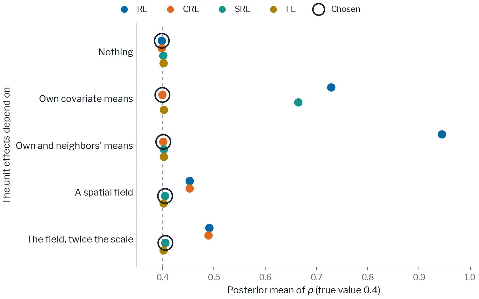
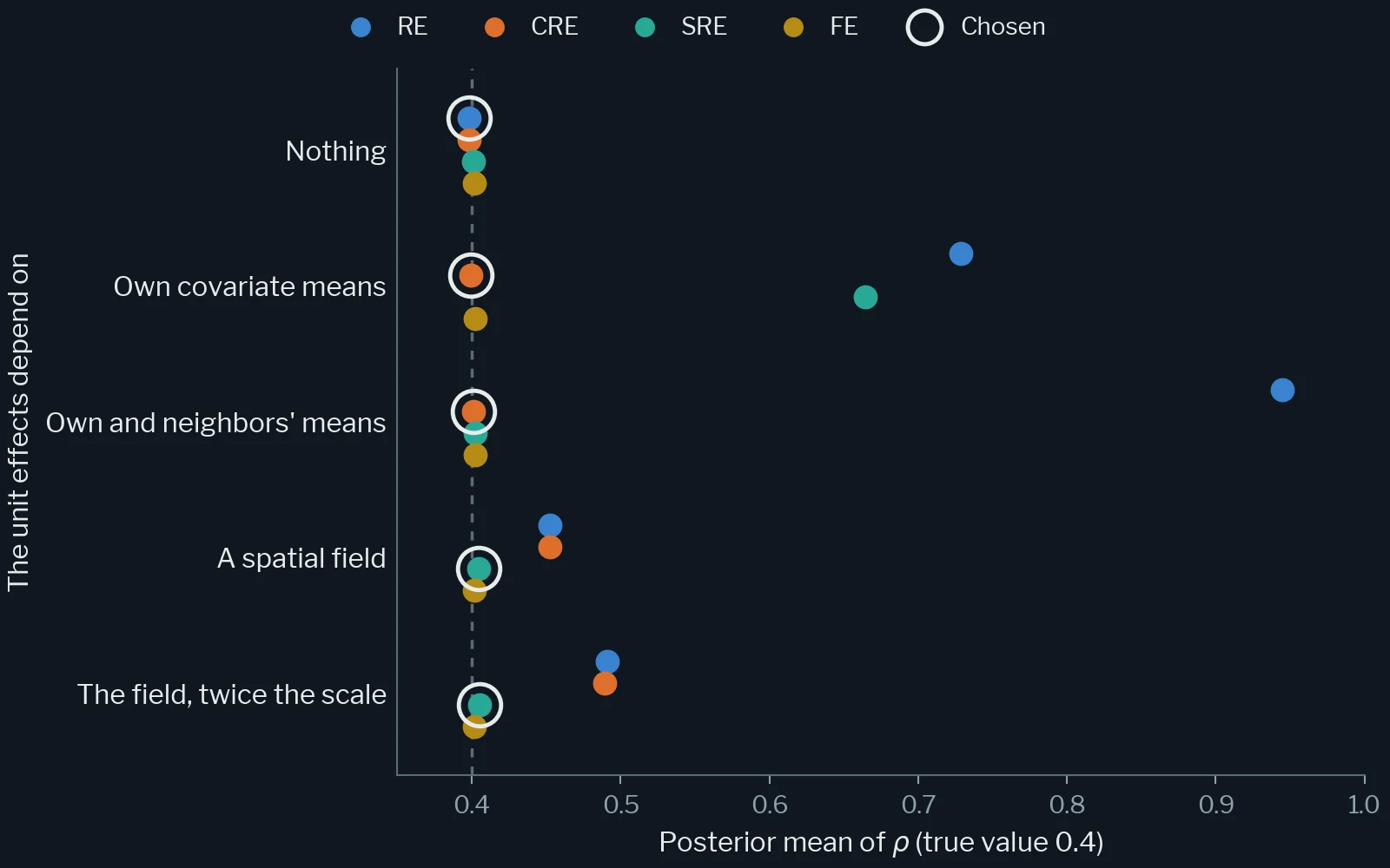
Whether a spatial panel’s unit effects are fixed or random decides which variation identifies its spatial parameter. The paper gives the analyst one Bayes factor that chooses among random, correlated random, spatially correlated random, and fixed effects, and that names the assumption at fault when random effects fail. The same comparison chooses between the spatial lag and spatial Durbin models, and with a complementary overidentification statistic it forms a specification search for spatial panels, beside the Lagrange-multiplier tests of the spatial process.
The usual arbiter is a Hausman contrast (Mutl and Pfaffermayr 2011; Lee and Yu 2012), whose alternative is effects correlated with the covariates. Spatial data admit a second departure: the effects of neighboring units can be correlated with one another, as when an unobserved condition spans several units. Under such effects random effects misstate the spatial parameter, and so does the Mundlak model, the alternative those tests take. A likelihood Bayes factor cannot settle the matter either, because fixed effects are random effects under a flat prior, and whoever sets the prior on the effects decides between them.
The paper compares the models by their moment conditions instead. Each random-effects assumption states that a block of moments is zero, and a model that drops an assumption frees its block, so the four models differ only in the blocks they free. Their marginal exponentially tilted empirical likelihoods need no prior on the effects, and under high-level conditions the comparison selects the most restrictive valid model with probability tending to one. On the county homicide panel of Baller and colleagues (2001), 3,085 U.S. counties in the censuses from 1960 to 1990, it chooses the spatial Durbin model with fixed effects.